TimescaleDB is a powerful open-source database designed to handle massive amounts of time-series data efficiently. It’s perfect for companies that need to store and analyze data over time, like IoT sensors, financial records, or scientific experiments. Time-series data has become increasingly important across many industries. Whether you’re tracking sensor data, monitoring system performance, or analyzing stock market trends, time-series databases have emerged as the go-to solution for managing and querying large amounts of data efficiently. This is where TimeScaleDB shines.
Built on top of PostgreSQL, it combines the flexibility, reliability, and familiarity of SQL with specific optimizations for time-series workloads, making it a highly scalable and efficient solution for real-time and historical data analysis.
In this blog, we’ll walk through the core functionalities of TimeScaleDB using an example from the financial sector: tracking stock market data. We’ll cover key concepts like hypertables, partitioning, chunking, data retention, and advanced query features like time bucketing and hyperfunctions. By the end, you’ll understand how to efficiently manage, query, and analyze large-scale stock data with TimeScaleDB.
Step-by-Step Example: Stock Market Data with TimeScaleDB
Step 1: Setting Up TimeScaleDB and Creating the Stock Prices Table
Let’s imagine you’re tracking stock price movements for multiple companies every minute. The data includes the stock’s timestamp, symbol, open price, close price, high, low, and volume traded.
We’ll start by installing TimeScaleDB (if you haven’t already). TimeScaleDB is a PostgreSQL extension, so make sure you have PostgreSQL installed and follow TimeScaleDB installation steps for your specific environment.
Once installed, let’s create a simple table for storing stock data:
    CREATE TABLE stock_data (
        time TIMESTAMPTZ NOT NULL,
        symbol TEXT NOT NULL,
        open_price DOUBLE PRECISION,
        close_price DOUBLE PRECISION,
        high_price DOUBLE PRECISION,
        low_price DOUBLE PRECISION,
        volume BIGINT
    );
Here’s a breakdown of the columns:
- time The timestamp when the data was recorded.
- symbol The stock’s symbol (e.g., AAPL for Apple, MSFT for Microsoft).
- open_price The stock’s opening price at a given time.
- close_price The stock’s closing price at that time.
- high_price/low_price The highest and lowest price within that time interval.
- volume The number of shares traded during that interval.
Step 2: Converting the Table to a Hypertable
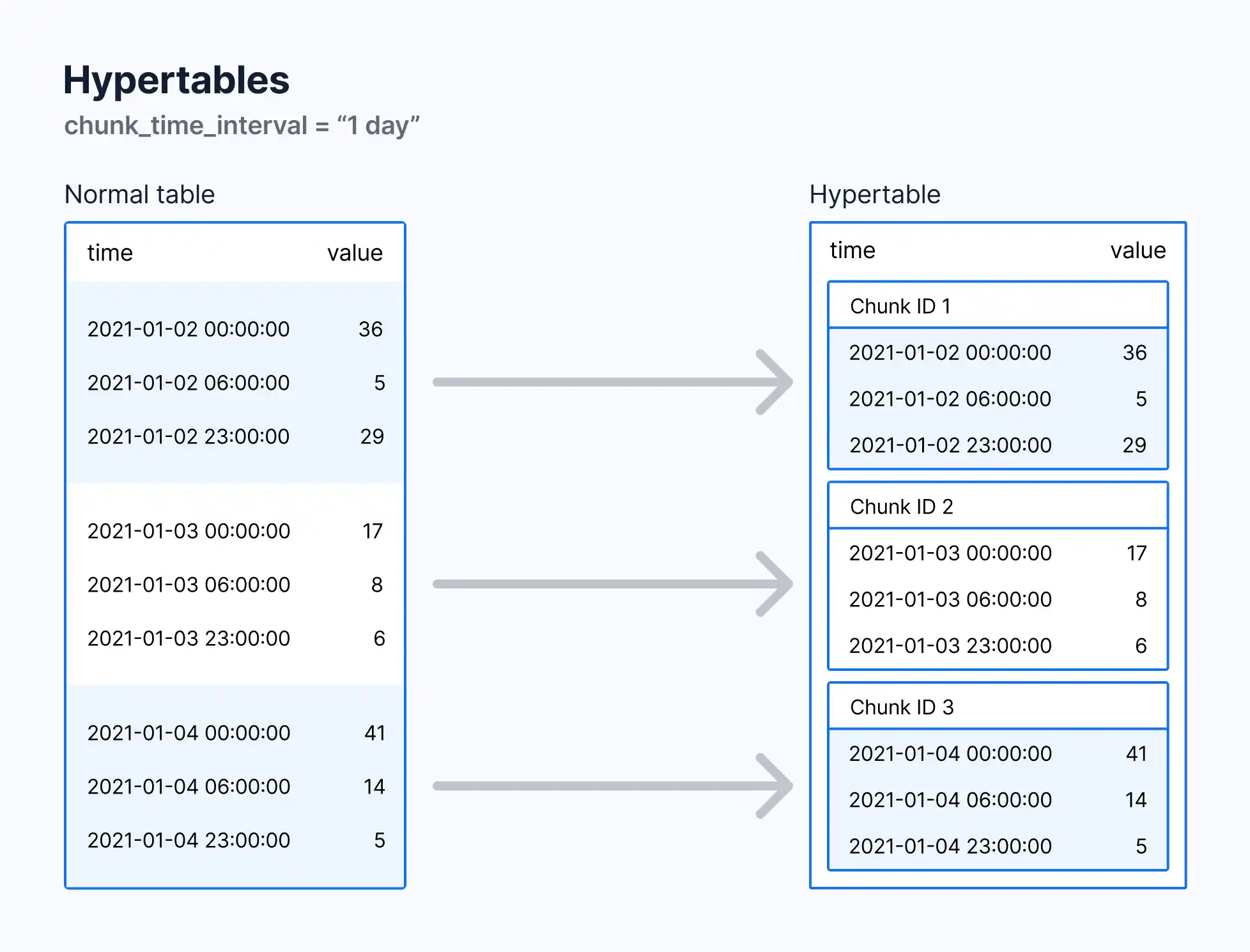
A hypertable is a special type of table in TimeScaleDB that automatically partitions your time-series data into smaller chunks for efficient querying and storage. To convert the stock_data table into a hypertable, run:
SELECT create_hypertable('stock_data', 'time');
In this case, the time column is our partition column because time-series data is naturally partitioned by time. This setup allows TimeScaleDB to automatically handle large volumes of data without manual intervention.
Column Partitioning in TimeScaleDB
Apart from partitioning based on time, TimeScaleDB allows for space partitioning—an additional partition based on another column besides time, typically used when dealing with datasets that include multiple data sources (e.g., different stock symbols). This improves performance, especially with large datasets.
In our stock market example, we could partition the table by both time and symbol. By doing so, TimeScaleDB will further optimize queries that filter by stock symbol, speeding up analysis for specific stocks:
SELECT create_hypertable('stock_data', 'time', 'symbol', number_partitions => 4);
Here, the symbol column is used for column partitioning, and the number of partitions is set to 4. This means the stock data is divided into four partitions, each managing different symbols, reducing query complexity for individual stocks.
Step 3: Customizing Chunking with chunk_time_interval
TimeScaleDB automatically breaks your time-series data into chunks, each covering a specific time period, which makes it faster to query and manage. You can control how much data each chunk holds using the chunk_time_interval setting.
For stock data that is being tracked every minute, we might want to create weekly chunks to balance the load between data ingestion and querying:
ALTER TABLE stock_data SET (timescaledb.chunk_time_interval = '7 days');
This configuration splits the data into weekly chunks, meaning each chunk will store one week’s worth of stock data. By doing this, queries that cover a weekly or daily interval are optimized, while reducing memory usage. Proper chunking ensures TimeScaleDB performs efficiently both for real-time data ingestion and querying historical data.

Why Use Chunking?
- Optimized Queries When querying a specific time range, only the relevant chunks are scanned, speeding up performance.
- Storage Efficiency Data is stored in smaller, manageable chunks, reducing I/O overhead.
- Flexibility The chunk_time_interval can be adjusted based on data frequency. For high-frequency data (like stock prices every minute), smaller chunk intervals (e.g., weekly or daily) are recommended.
Step 4: Managing Columns and Data Retention Policy
If you’re dealing with a massive amount of stock data, it’s common to retain highly granular data (like per-minute stock prices) only for a limited time. After a certain period, you can either delete or compress older data to save storage space. TimeScaleDB allows you to set up a retention policy for this purpose:
SELECT add_retention_policy('stock_data', INTERVAL '90 days');
This will automatically drop data older than 90 days from the stock_data table. This is especially useful in scenarios where you don’t need minute-level data from the past but would still like to keep aggregated data (e.g., daily or weekly summaries).
Step 5: Querying Data
Let’s see how you can query stock data efficiently using TimeScaleDB. You can retrieve the entire dataset for a specific symbol like so:
SELECT * FROM stock_data WHERE symbol = 'AAPL' AND time >= NOW() - INTERVAL '7 days';
But for time-series data, we often need aggregated information, like the average price or total volume traded over a specific time period. This is where TimeScaleDB’s hyperfunctions come in handy.
Step 6: Time-Interval Bucketing with time_bucket
The time_bucket function allows you to group data into fixed time intervals. For example, let’s say we want to analyze Apple’s stock data over the last week and aggregate it by 1-hour intervals:
    SELECT time_bucket('1 hour', time) AS bucket,
        AVG(close_price) AS avg_close,
        MAX(high_price) AS max_high,
        MIN(low_price) AS min_low,
        SUM(volume) AS total_volume
    FROM stock_data
    WHERE symbol = 'AAPL' AND time >= NOW() - INTERVAL '7 days'
    GROUP BY bucket
    ORDER BY bucket;
This query breaks the data into 1-hour buckets and aggregates the stock’s closing prices, highest price, lowest price, and volume traded for each interval.
Step 7: Advanced Aggregations with HyperFunctions
TimeScaleDB’s hyperfunctions, designed for advanced time-series analysis, can simplify complex queries and provide more insights. Let’s explore a few of these.
1. Moving Averages
In stock analysis, moving averages help smooth out price data to identify trends. You can compute a moving average on the stock’s closing price over the last 30 minutes using the time_bucket and moving_avg functions:
    SELECT time_bucket('1 minute', time) AS minute,
        moving_avg(close_price, 30) AS moving_avg_close
    FROM stock_data
    WHERE symbol = 'AAPL' AND time >= NOW() - INTERVAL '2 hours'
    GROUP BY minute
    ORDER BY minute;
2. Percentile Aggregation
To find how often a stock price closes above or below a certain threshold, you can use the percentile_agg function. For instance, to calculate the 90th percentile closing price for Apple stock over the last 7 days:
    SELECT approx_percentile(0.90, percentile_agg(close_price)) AS p90_close
    FROM stock_data
    WHERE symbol = 'AAPL' AND time >= NOW() - INTERVAL '7 days';
3. Downsampling Data with time_bucket_gapfill
When dealing with stock data, gaps in time (e.g., non-trading hours) can skew analysis. You can use the time_bucket_gapfill function to ensure continuous time intervals:
    SELECT time_bucket_gapfill('1 hour', time) AS bucket,
        locf(last(close_price, time)) AS last_close_price
    FROM stock_data
    WHERE symbol = 'AAPL' AND time >= NOW() - INTERVAL '7 days'
    GROUP BY bucket;
This query ensures that missing time intervals are “filled” with the last known value, which can be important for generating accurate reports over time.
Step 8: Putting It All Together
By using TimeScaleDB, you can manage massive datasets with ease, optimize storage, and write efficient queries that aggregate and analyze stock data quickly. Let’s summarize a typical workflow:
- Hypertable Creation We created a hypertable to store time-series stock data.
- Chunking and Column Partitioning We defined a chunk_time_interval to split data into manageable weekly chunks and used column partitioning to optimize queries based on stock symbols.
- Retention Policy We set a retention policy to automatically drop data older than 90 days.
- Time Bucketing We grouped stock data into hourly intervals for easier analysis using time_bucket.
- Advanced Aggregations We used TimeScaleDB hyperfunctions like moving_avg, percentile_agg, and time_bucket_gapfill to perform advanced time-series analytics.
Conclusion
TimeScaleDB offers powerful tools for managing and querying time-series data, especially in high-frequency use cases like stock trading. Its PostgreSQL compatibility, along with unique time-series optimizations, makes it ideal for financial data storage, retention, and real-time analytics. By utilizing hypertables, chunking, column partitioning, and hyperfunctions, you can build highly efficient and scalable stock market applications with ease.
Whether you’re monitoring IoT devices, financial markets, or application metrics, TimeScaleDB offers the functionality needed to store and analyze time-series data effectively. Give TimeScaleDB a try for your next time-series project!
